Brand Positioning by Correspondence Analysis
I was reading an article about visualization techniques using multidimensional scaling (MDS), the correspondence analysis in particular. The example used R, but as usual, I want to find ways to do it with Python, so here goes.
The correspondence analysis is useful when you have a two-way contingency table for which relative values of ratio-scaled data are of interest. For example, I here use a table where the rows are fashion brands (Chanel, Louis Vuitton, etc.) and the columns are the number of people who answered that the particular brand has the particular attribute expressed by the adjective (luxurious, youthful, energetic, etc.). (I borrowed the data from this article.)
The correspondence analysis (or MDS in general) is a method of reducing dimensions to make the data more sensible for interpretation. In this case, I get a scatter plot of brands and adjectives in two-dimensional space, in which brands/adjectives more closely associated with each other are placed near each other.
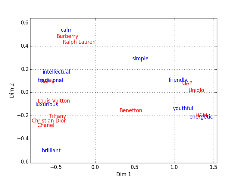
Figure 1: Brand Positioning
As you see, brands like GAP, H&M, and Uniqlo are associated with youth, friendliness, and energy, while old-school brands like Chanel and Tiffany are associated with luxury and brilliance. This way of visualization is useful because the high-dimensional information (11 brands and 9 attributes) is reduced into a two-dimensional plane, and the distance on that plane is meaningful.
Here’s the code and data (available also in Gist):
#!/usr/bin/env python2.7
# -*- coding: utf-8 -*-
import matplotlib.pyplot as plt
import numpy as np
from numpy.linalg import svd


class CA(object):
    """Simple corresondence analysis.

    Inputs
    ------
    ct : array_like

      Two-way contingency table. If `ct` is a pandas DataFrame object,
      the index and column values are used for plotting.

    Notes
    -----
    The implementation follows that presented in 'Correspondence
    Analysis in R, with Two- and Three-dimensional Graphics: The ca
    Package,' Journal of Statistical Software, May 2007, Volume 20,
    Issue 3.

    """

    def __init__(self, ct):
        self.rows = ct.index.values if hasattr(ct, 'index') else None
        self.cols = ct.columns.values if hasattr(ct, 'columns') else None

        # contingency table
        N = np.matrix(ct, dtype=float)

        # correspondence matrix from contingency table
        P = N / N.sum()

        # row and column marginal totals of P as vectors
        r = P.sum(axis=1)
        c = P.sum(axis=0).T

        # diagonal matrices of row/column sums
        D_r_rsq = np.diag(1. / np.sqrt(r.A1))
        D_c_rsq = np.diag(1. / np.sqrt(c.A1))

        # the matrix of standarized residuals
        S = D_r_rsq * (P - r * c.T) * D_c_rsq

        # compute the SVD
        U, D_a, V = svd(S, full_matrices=False)
        D_a = np.asmatrix(np.diag(D_a))
        V = V.T

        # principal coordinates of rows
        F = D_r_rsq * U * D_a

        # principal coordinates of columns
        G = D_c_rsq * V * D_a

        # standard coordinates of rows
        X = D_r_rsq * U

        # standard coordinates of columns
        Y = D_c_rsq * V

        # the total variance of the data matrix
        inertia = sum([(P[i,j] - r[i,0] * c[j,0])**2 / (r[i,0] * c[j,0])
                       for i in range(N.shape[0])
                       for j in range(N.shape[1])])

        self.F = F.A
        self.G = G.A
        self.X = X.A
        self.Y = Y.A
        self.inertia = inertia
        self.eigenvals = np.diag(D_a)**2

    def plot(self):
        """Plot the first and second dimensions."""
        xmin, xmax = None, None
        ymin, ymax = None, None
        if self.rows is not None:
            for i, t in enumerate(self.rows):
                x, y = self.F[i,0], self.F[i,1]
                plt.text(x, y, t, va='center', ha='center', color='r')
                xmin = min(x, xmin if xmin else x)
                xmax = max(x, xmax if xmax else x)
                ymin = min(y, ymin if ymin else y)
                ymax = max(y, ymax if ymax else y)
        else:
            plt.plot(self.F[:, 0], self.F[:, 1], 'ro')

        if self.cols is not None:
            for i, t in enumerate(self.cols):
                x, y = self.G[i,0], self.G[i,1]
                plt.text(x, y, t, va='center', ha='center', color='b')
                xmin = min(x, xmin if xmin else x)
                xmax = max(x, xmax if xmax else x)
                ymin = min(y, ymin if ymin else y)
                ymax = max(y, ymax if ymax else y)
        else:
            plt.plot(self.G[:, 0], self.G[:, 1], 'bs')

        if xmin and xmax:
            pad = (xmax - xmin) * 0.1
            plt.xlim(xmin - pad, xmax + pad)
        if ymin and ymax:
            pad = (ymax - ymin) * 0.1
            plt.ylim(ymin - pad, ymax + pad)

        plt.grid()
        plt.xlabel('Dim 1')
        plt.ylabel('Dim 2')

    def scree_diagram(self, perc=True, *args, **kwargs):
        """Plot the scree diagram."""
        eigenvals = self.eigenvals
        xs = np.arange(1, eigenvals.size + 1, 1)
        ys = 100. * eigenvals / eigenvals.sum() if perc else eigenvals
        plt.plot(xs, ys, *args, **kwargs)
        plt.xlabel('Dimension')
        plt.ylabel('Eigenvalue' + (' [%]' if perc else ''))


def _test():
    import pandas as pd

    df = pd.io.parsers.read_csv('data/fashion_brands.csv')
    df = df.set_index('brand')

    print df.describe()
    print df.head()

    ca = CA(df)

    plt.figure(100)
    ca.plot()

    plt.figure(101)
    ca.scree_diagram()

    plt.show()


if __name__ == '__main__':
    _test()
The data in the CSV format used for the analysis:
brand,luxurious,traditional,intellectual,brilliant,calm,youthful,friendly,simple,energetic
Chanel,449,252,106,236,61,13,8,29,16
Louis Vuitton,410,286,83,142,80,18,20,48,31
Christian Dior,356,200,95,206,67,19,18,27,9
Tiffany,362,219,103,187,59,55,36,35,10
Rolex,442,248,114,89,109,4,9,52,12
Burberry,287,287,143,42,199,29,67,124,9
Ralph Lauren,198,191,101,39,147,61,70,100,9
Benetton,86,62,31,88,35,216,97,65,21
Uniqlo,6,7,10,8,23,260,331,199,291
H&M,8,5,10,2,10,272,132,91,223
GAP,10,10,10,9,24,275,203,137,84